Here is a new video on the Quadbot:
You may notice a mention of the RealSense depth camera towards the end. More on this coming soon!
Here is a new video on the Quadbot:
You may notice a mention of the RealSense depth camera towards the end. More on this coming soon!

Some good news for the quadruped project, as I entered it into the Human Computer Interface Challenge, part of the larger 2018 Hackaday Prize contest, and it was one of the 20 winners!
Here are the links to the announcement and highlight articles:

I added some exponential smoothing to the original walking gaits, to smooth the edges of the trajectories and create a more natural movement.
I then added a ±30° pitching motion to what best approximates the ‘ankle’ (4th joint), to emulate the heel off and heel strike phases of the gait cycle.
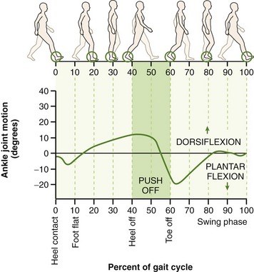
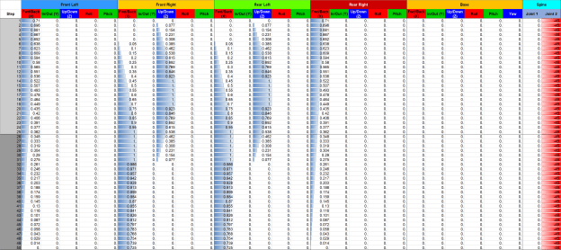
The range of motion of the right ankle joint. Source: Clinical Gate.
I realised however that applying the pitch to the foot target is not exactly the same as applying the pitch to the ankle joint. This is because, in the robot’s case, the ‘foot target’ is located at the centre of the lowest part of the foot, that comes into contact with the ground, whereas the ankle is higher up, at a distance of two link lengths (in terms of the kinematics, that’s a4+a5). The walking gait thus does not ends up producing the expected result (this is best explained by the animations are the end).
To account for this, I simply had to adjust the forward/backward and up/down position of the target, in response to the required pitch.
With some simple trigonometry, the fwd/back motion is adjusted by 
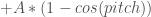

Here are the details showing how the targets are adjusted for one particular phase in the creep walk gait (numbers involving translations are all normalised because of the way the gait code currently works):
Creep walk gait, 25-step window where the foot target pitch oscillates between ±30°. Original target translations (fwd/back, up/down) are shown compared to the ones adjusted in response to the pitch.
The final results of the foot pitching, with and without smoothing, are shown below:

Following on from the previous post on walking and steering, I realised that when moving the spine joints, the rear feet remain anchored to the ground, when it would be better if they rotated around the spine motors, to give a better turning circle for steering.
The reason behind why the feet remain fixed is because their targets are being defined in world coordinate space, so moving the spine won’t change the target.
There are advantages to defining the targets in world space for future work, when the robot knows more information about its environment. For example the legs can be positioned in the world in order to navigate upcoming terrain or obstacles. But for now, it is often useful to work in coordinates local to the base (front base for front legs, and rear base for rear legs), since in this way you don’t have to worry about the relative positioning of the front base w.r.t. rear.
I will eventually update the kinematics code so either world or local targets can be selected.
For now however, I have made an update to the code, so if the spine joint sliders, gaits or walking/steering inputs are used, the rear leg targets move with the spine. To explain this better visually:
Another minor adjustment you might notice was the widening of the stance, to provide a larger support polygon. The walking gaits still need fine-tuning, as walking on the actual robot is still unstable and slow.

Some slow progress lately, but progress nonetheless. First, I have updated the walking gaits with additional target values. Second, I have added a new input mode which allows the predefined walking gaits to be scrolled through via the keyboard or controller inputs. In effect, this means the controller can be used to “remote-control” the walking of the robot! The walking gaits still need a lot of tuning, but the basic function is now implemented.
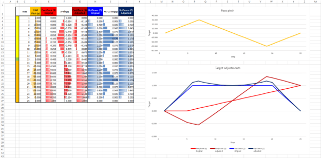
I have updated the CSV spreadsheet for gait data, so that it now includes the 5 possible degrees-of-freedom of each foot (XYZ and Roll/Pitch), the 6 DoF of the base, and the 2 spine joints.
The walking gait’s updated list of foot target values (first 50 out of 100).

The foot target values visualised (base and spine joints not shown).
In Python, all the CSV data is loaded into an array. One of the keyboard/controller inputs can now also be used to update an index, that scrolls forwards/backwards through the array’s rows.
Next, to get the robot to turn, a second input controls a deflection value which adjusts one of the spine joints and the base orientation (as was mentioned in this past post). The deflection slowly decreases back to 0, if the input is also 0.
By doing this, the walking gait can be controlled at will by the two inputs, and hopefully make the robot walk and turn. Next comes the fine-tuning and testing!
All the latest code can be found on the Quadbot17 GitHub project page as usual.
New video!
I have been testing the movement of the robot’s base in the world, while keeping the legs fixed to the ground, as a test of the robot’s stability and flexibility.
The robot base can now be controlled, either via the GUI, keyboard or gamepad, in the following ways:
You may notice the real robot can’t move its upper leg all the way horizontally as the IK might suggest is possible, because there is a small clash between the AX-12 and the metal bracket, but this should be fixed by filing or bending the curved metal tabs:
I have recently written an OpenCM sketch to control the robot servos, in a way similar to how it was being done with the older Arbotix-M, but this time using the Robotis libraries for communicating with the motors.
I have also been making various updates to the Python test code, with a few of the main issues being:
All the latest code can be found on the Quadbot17 GitHub project page as usual.

Over the last few weeks I have been thinking about the overall controller architecture, 3D printing some test Raspberry Pi cases, and updating the Python test software.
After refactoring the giant single-file script from the previous post, I noticed the script was actually running very inefficiently, partly down to the fact that the 2D canvas had to redraw the whole robot on every frame, but also because of the way some of the threaded classes (e.g. input handler, serial handler) were inadvertently constantly interrupting the main thread, because they were relying on use of the root window’s after() method. The timing loops are cleaned up now and the code runs much more efficiently.
Here is an example I figured out, of how to create a class to run a function in a separate thread, with a defined time interval, that is pausable/stoppable. It subclasses the Thread class, and uses the help of an Event object to handle the timing functionality. After creating an object of this class, you call its start() method, which invokes the run() method in a separate thread. The pause(), resume() and stop() methods perform the respective actions. The example is a stripped-down version of an input handler, which applies the equations of motion to user inputs, as shown in a past post.
import threading
from time import time
import math
class InputHandlerExample(threading.Thread):
    def __init__(self):
        # Threading/timing vars
        threading.Thread.__init__(self)
        self.event = threading.Event()
        self.dt = 0.05  # 50 ms
        self.paused = False
        self.prevT = time()
        self.currT = time()
        self.target = 0.0
        self.speed = 0.0

        # Input vars
        self.inputNormalised = 0.0

    def run(self):
        while not self.event.isSet():
            if not self.paused:
                self.pollInputs()
            self.event.wait(self.dt)

    def pause(self):
        self.paused = True

    def resume(self):
        self.paused = False

    def stop(self):
        self.event.set()

    def pollInputs(self):
        # Upate current time
        self.currT = time()

        # Get user input somehow here, normalise value
        #self.inputNormalised = getInput()

        # Update target and speed
        self.target, self.speed = self.updateMotion(
            self.inputNormalised, self.target, self.speed)

        # Make use of the returned target and speed values
        #useResults(target, speed)

        # Update previous time
        self.prevT = self.currT

    def updateMotion(self, i, target, speed):
        m = 1.0
        u0 = speed

        # Force minus linear drag
        inputForceMax = 1000
        dragForceCoef = 5
        F = inputForceMax*i - dragForceCoef*u0
        a = F/m
        t = self.currT - self.prevT

        # Zero t if it's too large
        if t > 0.5:
            t = 0.0
        x0 = target

        # Equations of motion
        u = u0 + a*t
        x = x0 + u0*t + 0.5*a*math.pow(t, 2)

        return x, u
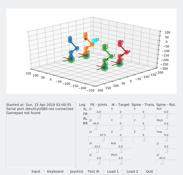
So far the 2D representation of the robot worked OK, but it has its limitations. So I finally decided to put some effort into updating the representation of the robot. I went with matplotlib and its 3D extensions with the mplot3d toolkit.
The joints are simply represented using the scatter() function, while the lines are simply drawn with plot(). The text() function overlays the number of the joints over the joint positions. The leg target widgets use a combination of the above functions. The 3D plot is updated using the FuncAnimation class.
Since this designed for Matlab-style plotting rather than a simulator, the performance is still somewhat lacking (not as fast as the 2D canvas), but I wanted to be able to get something working fairly quickly and not waste too much time with something like OpenGL, since my aim is to have a test program and not build a 3D simulator from scratch. There’s always ROS and Gazebo if I need to take this further!
As a side note, I have added the option in the main program to be able to select between 2D or 3D drawing mode, as well as no drawing, which should be useful for speeding up execution when running on the Raspberry Pi in headless mode (no screen).
Here is a screenshot and a video of the results:
Another efficiency issue was the fact that previously the canvas was cleared an then redrawn from scratch on every frame update. To improve efficiency, both for the 2D and the 3D cases, the drawing classes now have structs to keep track of all element handles, and the redraw functions move the elements to their updated positions. For the 2D case (TkInter canvas), this is done with the coords() method. For the 3D case (matplotlib) it was a bit trickier, but I managed it with a combination of methods:
The interaction between the different elements is cleaned up and now looks like this:

Now, to make a switch and talk a bit more about the hardware, here is the current plan of how all the components will probably look like:

I have in fact got two Raspberry Pis now, a Pi 3 Model B as well as a Pi Zero W. Both now have built-in WiFi, but I am going with the larger Pi 3 as the current choice for main controller, favouring the quad-core CPU over the Zero’s single core.
I tried 3D printing some cases from Thingiverse for each Pi, and here are the results. A great plus point of the Pi 3 case is that it has mounting points which will be easy to locate on the main robot body.


You can find my builds and their sources on Thingiverse:
Here is a quick update on current progress with the software:

Latest test program, with keyboard input and full spine control.
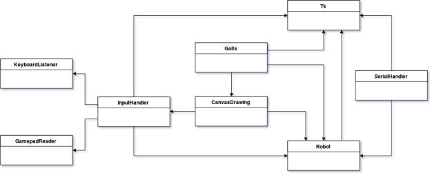
Simple class diagram of the Python program, after refactoring the original single-file script.
On the hardware side, I have some new controllers to explore various ideas, namely a Robotis OpenCM9.04 and a Raspberry Pi 3. The Raspberry could be mounted to the robot with a 3D-printed case like this.
After 3D printing a few more plastic parts and cutting all the aluminium plates, the custom chassis is finally complete! Below are some quick notes on the progress over the last weeks.
I printed off some of the remaining parts of the chassis. The battery compartment was best printed upright with minimal support structure needed. The rear bumper was trickier than the front bumper, because of the additional hole space for the battery, so I found it was best to print upright, with a raft and curved supports at the bottom.
Once all parts were printed, and some more sanding, I spray-painted all the parts with plastic primer, then blue paint, and finally clear sealer.


I was initially thinking of finding an online service to cut out the aluminium chassis parts, but then decided it would be faster and cheaper to just get some sheets 1.5 mm thick aluminium sheets from eBay and cut them on a jigsaw table.
I used Fusion 360’s drawing tool to export to PDF the parts I needed to cut out: four chassis plates and four foot plates. I then printed them in actual scale and glued them on the aluminium to uses as traces.


I threaded the holes on all the 3D parts, which were either 3 mm wide where the aluminium plates attach, or 2 mm at the leg and spine bracket attachment points.
Using a tap for the 3 mm holes worked pretty well, but the 2 mm holes were more prone to being stripped or too loose, so manually threading the holes with the bolts worked better. Another issue was the infill surrounding the internal thread cylinder sometimes being a bit too thin. In retrospect, I’d try designing the 3D parts to use heat-set or expandable inserts, especially for the smaller threads.
The servo brackets attaching to the chassis have a large number of holes (16 for each leg and one of the spine brackets, and 12 for the other spine bracket) so the screws so far seem to secure the brackets well enough. The spine section is under a lot of stress from the wight of the whole chassis and legs, so it will not be able to withstand much twisting force, and the servos may not be strong enough at this area, but I will have to test this in practice with new walking gaits.


The custom chassis has finally made it from a 3D design to a reality, with relative success so far. Some of the threaded holes on the 3D parts are not as strong as I’d like, the AX-12 may be under-powered for the spine connection, and the brackets anchoring the spine may be the first to give way due to twisting forces. Also the chassis as a whole would benefit form weight-saving exercise and perhaps being thinned down. But this has only been the first iteration of the main chassis, and the robot design has now become a reality and seems to stand up well. The next step will see how it performs some of the basic walking gaits!

… or more correctly, from CAD to reality, as it is time for 3D printing!
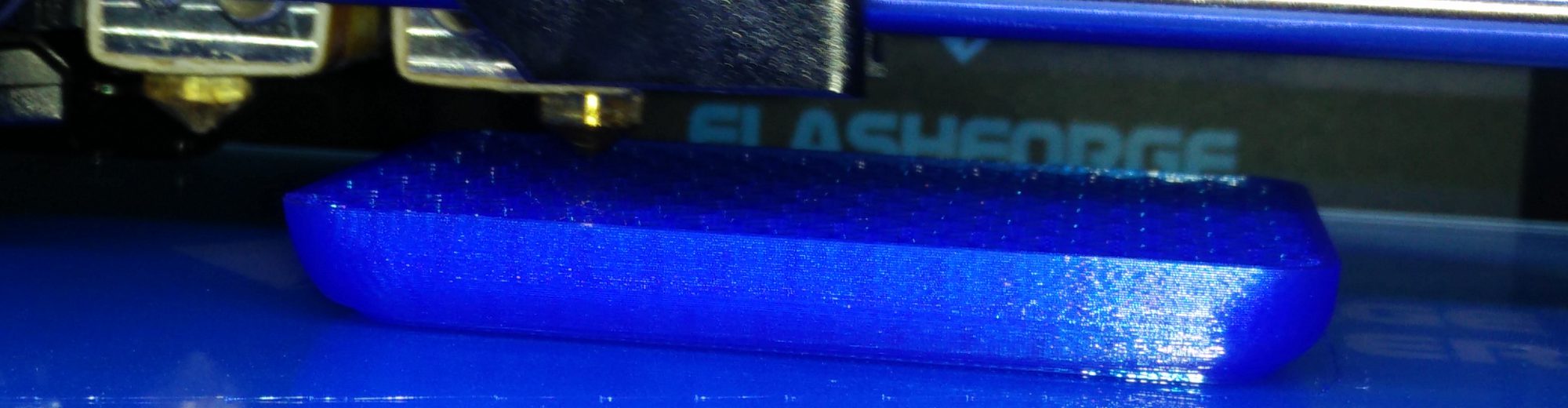
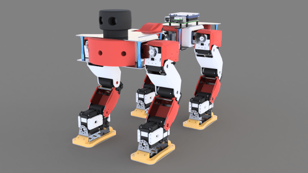
I’ve recently got a new 3D printer in the form of a FlashForge Creator Pro 2017, which means I can start printing some of the structural components for the quadruped now, leaving the decorative pieces for later. In fact, some of them have already been printed, as you can see in the images below.
All the parts were recently updated from their previous iteration slightly, by adding fillets around the edges, and decreasing nut hole diameters by 0.2 mm in order to provide some material for self-tapping threads. On the other hand, I increased the tolerance of some slots by the same amount, to allow a tolerance for their connection to interlocking plastic tabs.
The rear section has also been modified: the underside aluminium base will have a tab at 90° that connects to the rear, to provide more rigidity to the central connection with the spine servo bracket.
Here are the CAD models of the chassis parts:


All parts were printed in PLA plastic.
The first part I started with was the foot base. I printed it with a 20% honeycomb infill. I didn’t add any intermediate solid layers, but might do so in other parts. I have so far printed two out of the four bases.
Each leg will connect to a leg base bracket, which is the same design for all legs. The part was printed “upside-down” because of the orientation of the interlocking tabs. This meant that some support structure was needed for the holes. For the first print attempt I also added supports around the overhang of the filleted edge, along with a brim, but for the subsequent prints I didn’t bother with these, as the fillet overhang held fine without supports, and saved from extra filing/sanding down. These parts also used 20% infill.
For the front and rear “bumpers”, I reduced the infill to 10%.
For the larger part comprising of the central section of the front, the spine front bracket, I also used an infill of 10%. Due to the more complicated design that would have included many overhangs, I found it easier to cut the part lengthwise and print it as two separate pieces. These will be super-glued together after sanding.
Time-lapse GIFs and images of the printing process:

 854x480")


In terms of printing times, the foot bases and leg base brackets took about 3 hours each, the bumpers took around 4 hours each, and the two spine front bracket halves took about 7 hours combined, so total printing time is going to be fairly large!
The 0.2 mm clearance seems to work fine for self-threading the plastic with M2 size metal nuts, but was too large for some of the plastic-to-plastic interlocking tabs, possibly since this tolerance is close to the resolution limits of the printer (theoretically a 0.4 mm nozzle and 0.18 mm layer height). However after some filing and sanding down, all the plastic parts fit together nicely.
The resulting 3D prints before and after sanding:


Finally, here are some images of how the chassis assembly is shaping up, as well as the foot bases shown attached to the foot metal brackets. These fitted snug without any sanding, and all the holes aligned perfectly with the metal brackets, which was reassuring!


The next step is to glue the front bracket halves together, and maybe spray paint all the parts, as they lose all their original shine and end up looking very scratched after sanding.

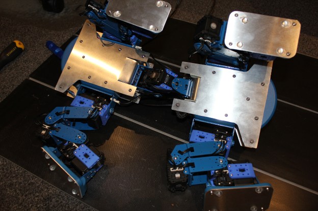
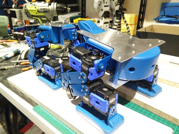
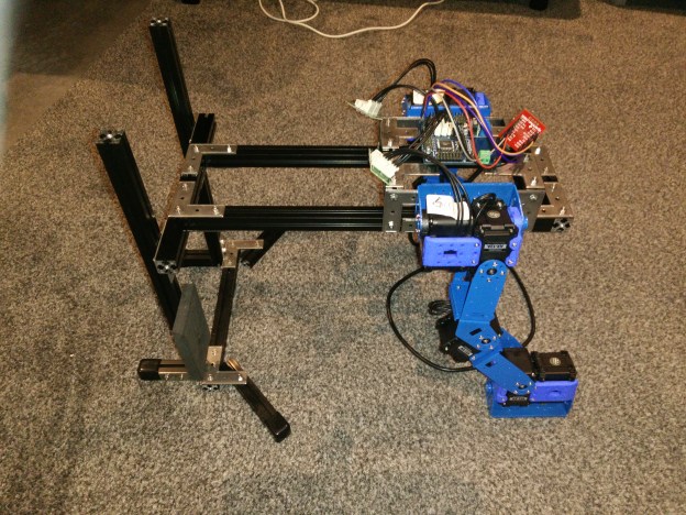
With the hardware for all four legs gathered, I have assembled the first standalone version of the quadruped. The MakerBeam XL aluminium profiles were adopted as before, to create a temporary chassis.
The fact that the robot can now stand on its four feet meant I could quickly give the walking gaits a test on the real hardware: The Python test software reads the up/down and forward/back position of each leg for a number of frames that make up a walking gait, the IK is solved, and the resulting joint values are streamed via serial over to the Arbotix-M, which simply updates the servo goal positions. No balancing or tweaking has been done whatsoever yet, which is why in the video I have to hold on to the back of the robot to prevent it from tipping backwards.
I took some time to make a video of the progress so far on this robot project:
A chance for some new photos:


Finally, here is an older video showing the Xbox One controller controlling the IK’s foot target position, and a simple serial program on the ArbotiX-M which receives the resulting position commands for each motor (try to overlook the bad video quality):
In the next stage I will start building the robot’s body, as per the CAD design, which is for the most part 3D printed parts and aluminium sheets, combined with the 2 DoF “spine” joints.
The Python test program has been updated to include the additional spine joints, transformation between the robot and world coordinates, and leg targets which take orientation into account.
This test script is used in anticipation for controlling the actual robot’s servos.
The “spine” consists of two joints which will allow the front of the robot to pitch and yaw independently of the rear. This will give it more flexibility when turning and handling uneven terrain, as well as other tasks such as aiming its sensors at the world.
Since the spine joints are quite simple, I don’t think there is any need to create IK for this section.
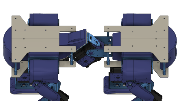
The “spine” joints separate the body of the quadruped between mostly similar front and rear sections.
The robot body now takes into account that it has to be oriented w.r.t. the “world”. This will be physically achieved by the information acquired by an IMU sensor. If the robot is tilted forwards, the targets for the legs will have to be adjusted so that the robot maintains its balance.
I have defined the kinematics in a way that if the the robot was to rotate w.r.t. the world, the whole body rotates (this can be achieved by moving the test Roll/Pitch/Yaw sliders). However if the servo joints of the spine are moved (test joint 1 / joint 2 sliders) the rear section of the robot will move w.r.t the world, and the rear legs will move with it, while the front section won’t change w.r.t. the world.
In order to achieve this, the leg IK had to be updated so that now the base frames of the front legs are linked to the front section of the robot, and the base frames of the rear legs are linked to the rear section.
You might notice while orientation will be defined by an IMU, pure translation (movement in XYZ) in the world is not considered for now, as it is meaningless without some sort of localisation capability in place. This could be achieved by a sensor (see below), but is an entirely separate challenge for a long way down the line (hint: SLAM).

New leg targets: Foot roll/pitch can be attained (within limits). In addition, the robot base can be positioned with respect to an outside world frame.

Original leg targets: The feet are always pointing vertical to the ground.
Initially, the leg target was simply a position in 3D for the foot link, and the foot was always pointing perpendicular to the ground, which made the inverse kinematics fairly easy. In version 2, the target orientation is now also taken into account. Actually, the pitch and roll can be targeted, but yawing cannot be obtained, simply because of the mechanics of the legs. Yawing, or turning, can be done by changing the walking gait pattern alone, but the idea is that the spine bend will also aid in steering the robot (how exactly I don’t know yet, but that will come later!).
Getting the kinematics to work were a bit trickier than the original version, mainly because the “pitching” orientation of the leg can only be achieved by the positioning of joint 4, whereas the “rolling” orientation can only be achieved by the positioning of joint 5. The available workspace of the foot is also somewhat limited, in part due to that missing yaw capability. Particularly at positions when the leg has to stretch sideways (laterally) then certain roll/pitching combinations are impossible to reach. Nevertheless, this implementation gives the feet enough freedom to be placed on fairly uneven surfaces, and not be constrained to the previously flat plane.
The next challenge that follows from this, is how can realistic target positions and orientations be generated (beyond predetermined fixed walking gaits), to match what the robot sees of the world?
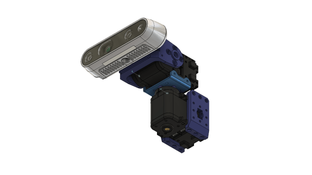
To answer this, first I need to decide how the robot sees the world: Primarily it will be by means of some 3D scanner, such as the ones I’ve looked into in the past, or maybe the Intel RealSense ZR300 which has recently caught my attention. But this alone might not be sufficient, and some form of contact sensors on the feet may be required.
The big question is, should I get a RealSense sensor for this robot ??? 🙂
Updated code can be found on GitHub (single-file test script is starting to get long, might be time to split up into class files!).

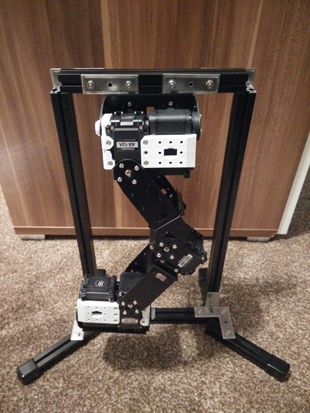
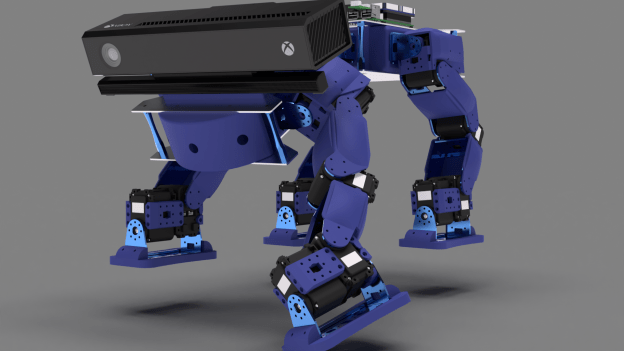
With enough motors and brackets to build a second leg, the hardware build continues! I have spray-painted all the metal brackets to go with an all-blue colour scheme. The Robotis plastic brackets were hard to source online, so I got them printed by Shapeways.
I re-purposed the test rig frame used for the single leg to make a platform for the two legs. It’s made out of MakerBeam XL aluminium profiles which are very easy to change around and customise to any shape. This base will work well until I get the rest of the plastic parts 3D printed and the metal parts cut.
I also had enough parts and motors to assemble the 2-axis “spine”, but the main frame is not yet built so it that part is on the side for now.
Here are a few photos of the build:


In the next post I will concentrate on software updates to the leg and spine kinematics.
I have updated the quadruped kinematics program to display all four legs and calculate their IK. I have also started working on the ways various walking gates can be loaded and executed. I found an interesting creeping walk gait from this useful quadruped robot gait study article, and replicated it below for use with my robot:

As you can see, the patterns are replicated in quadrants, in order to complete a full gait where each leg is moved forward once. In my test program, I use the up/down and forward/back position of each leg, to drive the foot target for each leg, as was done previously with the GUI sliders and gamepad.
The lateral swing of each leg (first joint) is not changed, but this can be looked at later. The “ankle” (last two joints) is controlled such that the leg plane is always parallel to the ground.
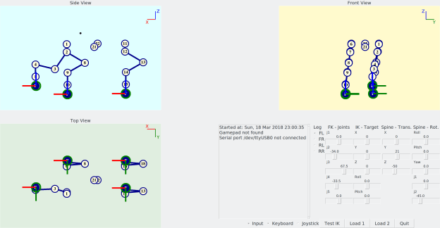
This is what the current state of the program looks like:
The foot target values are loaded from a CSV into the Python program, and the IK is run for each leg, going through the whole gait sequence:

I have also added the option to interrupt and run another gait sequence at any point. The reason for this is to try and experiment how to best switch or blend from one gait to another. For now, if a new gait is loaded, the program will stop the current gait, and compare the current pose to all poses in the new gait. The new gait will then start at the pose which most closely matches the current pose, by using a simple distance metric.
If the 8 values of up/down/fwd/back for all legs are in an array LastPose for the last pose the robot was in, and CurrPose for the current pose of interest from the new gait, then the pseudocode looks something like this:
DistanceMetric = 0
for i = 0 to 7
{
  d[i] = abs(CurrPose[i] - LastPose[i])
  if d[i] > threshold
  d[i] += penalty
  DistanceMetric += d[i]
}
If the distance in any particular direction is larger than some threshold, then an arbitrary penalty value can be added. This will bias the calculation against outliers: a pose with evenly distributed distances will be preferred over a pose with an overall small distance but large distance in one direction. This may not actually be of much use in practice, but can be tweaked or removed later.
The above pose switching idea will be expanded on, so that the robot can seemlessly blend between predefined walking gaits, e.g. when in order to turn left and right or speed up and down.
The next step is to start porting all this test code onto the Arbotix, which has a few minor challenges: Ideally the IK matrix operations need to be done efficiently without extra overhead from additional libraries. The gait values which are loaded from a CSV file need to be hard-coded, however this should be simple to do, since as shown above a gait uses the same target values rearranged across quadrants.
Until next time!

Seems like it’s Quadbot’s turn today. Project featured on the Fusion 360 community gallery, which means I need to hurry up and get it built.
The hardware for the test rig has arrived, and the first leg has been set up!
The metal brackets are from Trossen Robotics and largely match the dimensions of their equivalent plastic parts from Robotis. Some parts do not have metal counterparts, so I used spare plastic parts from my Bioloid kit. I also ordered an ArbotiX-M controller (Arduino-based), which communicates with the PC via a spare SparkFun FT232RL I had. The test rig frame is made out of MakerBeam XL aluminium profiles.
Unfortunately, I thought I had more 3-pin cables than I actually did, so I can’t control all the motors just yet. However, I’ve got an Xbox One controller controlling the IK’s foot target position and a simple serial program on the ArbotiX-M which receives the resulting position commands for each motor.


The code for both the Python applet and the Arduino can be found on GitHub here.
Some of the more useful snippets of code are shown below:
The following code handles gamepad inputs and converts them to a natural-feeling movement, based on equations of motion. The gamepad input gets converted into a virtual force, which is opposed by a drag proportional to the current velocity. The angles resulting from the IK are sent to the controller via serial port:
class GamepadHandler(threading.Thread):
    def __init__(self, master):
        self.master = master
        # Threading vars
        threading.Thread.__init__(self)
        self.daemon = True  # OK for main to exit even if instance is still running
        self.paused = False
        self.triggerPolling = True
        self.cond = threading.Condition()
        # Input vars
        devices = DeviceManager()
        self.target = targetHome[:]
        self.speed = [0, 0, 0]
        self.inputLJSX = 0
        self.inputLJSY = 0
        self.inputRJSX = 0
        self.inputRJSY = 0
        self.inputLJSXNormed = 0
        self.inputLJSYNormed = 0
        self.inputRJSXNormed = 0
        self.inputRJSYNormed = 0
        self.dt = 0.005

    def run(self):
        while 1:
            with self.cond:
                if self.paused:
                    self.cond.wait()  # Block until notified
                    self.triggerPolling = True
                else:
                    if self.triggerPolling:
                        self.pollInputs()
                        self.pollIK()
                        self.pollSerial()
                        self.triggerPolling = False
            # Get joystick input
            try:
                events = get_gamepad()
                for event in events:
                    self.processEvent(event)
            except:
                pass

    def pause(self):
        with self.cond:
            self.paused = True

    def resume(self):
        with self.cond:
            self.paused = False
            self.cond.notify()  # Unblock self if waiting

    def processEvent(self, event):
        #print(event.ev_type, event.code, event.state)
        if event.code == 'ABS_X':
            self.inputLJSX = event.state
        elif event.code == 'ABS_Y':
            self.inputLJSY = event.state
        elif event.code == 'ABS_RX':
            self.inputRJSX = event.state
        elif event.code == 'ABS_RY':
            self.inputRJSY = event.state

    def pollInputs(self):
        # World X
        self.inputLJSYNormed = self.filterInput(-self.inputLJSY)
        self.target[0], self.speed[0] = self.updateMotion(self.inputLJSYNormed, self.target[0], self.speed[0])
        # World Y
        self.inputLJSXNormed = self.filterInput(-self.inputLJSX)
        self.target[1], self.speed[1] = self.updateMotion(self.inputLJSXNormed, self.target[1], self.speed[1])
        # World Z
        self.inputRJSYNormed = self.filterInput(-self.inputRJSY)
        self.target[2], self.speed[2] = self.updateMotion(self.inputRJSYNormed, self.target[2], self.speed[2])
        with self.cond:
            if not self.paused:
                self.master.after(int(self.dt*1000), self.pollInputs)

    def pollIK(self):
        global target
        target = self.target[:]
        runIK(target)
        with self.cond:
            if not self.paused:
                self.master.after(int(self.dt*1000), self.pollIK)

    def pollSerial(self):
        if 'ser' in globals():
            global ser
            global angles
            writeStr = ""
            for i in range(len(angles)):
                x = int( rescale(angles[i], -180.0, 180.0, 0, 1023) )
                writeStr += str(i+1) + "," + str(x)
                if i  3277) or (i  3277:
                oldMax = 32767
            elif i < -3277:
                oldMax = 32768
            inputNormed = math.copysign(1.0, abs(i)) * rescale(i, 0, oldMax, 0, 1.0)
        else:
            inputNormed = 0
        return inputNormed

    def updateMotion(self, i, target, speed):
        c1 = 10000.0
        c2 = 10.0
        mu = 1.0
        m = 1.0
        u0 = speed
        F = c1*i - c2*u0  # Force minus linear drag
        a = F/m
        t = self.dt
        x0 = target
        # Equations of motion
        u = u0 + a*t
        x = x0 + u0*t + 0.5*a*pow(t, 2)
        # Update self
        target = x
        speed = u
        return target, speed

def rescale(old, oldMin, oldMax, newMin, newMax):
    oldRange = (oldMax - oldMin)
    newRange = (newMax - newMin)
    return (old - oldMin) * newRange / oldRange + newMin
The following Python code is the leg’s Forward Kinematics (click to expand):
def runFK(angles):
    global a
    global footOffset
    global T_1_in_W
    global T_2_in_W
    global T_3_in_W
    global T_4_in_W
    global T_5_in_W
    global T_F_in_W

    a = [0, 0, 29.05, 76.919, 72.96, 45.032]  # Link lengths "a-1"

    footOffset = 33.596

    s = [0, 0, 0, 0, 0, 0]
    c = [0, 0, 0, 0, 0, 0]
    for i in range(1,6):
        s[i] = math.sin( math.radians(angles[i-1]) )
        c[i] = math.cos( math.radians(angles[i-1]) )

    # +90 around Y
    T_0_in_W = np.matrix( [ [  0,  0,  1,  0],
                            [  0,  1,  0,  0],
                            [ -1,  0,  0,  0],
                            [  0,  0,  0,  1] ] )

    T_1_in_0 = np.matrix( [ [ c[1], -s[1],  0, a[1]],
                            [ s[1],  c[1],  0,    0],
                            [    0,     0,  1,    0],
                            [    0,     0,  0,    1] ] )

    T_2_in_1 = np.matrix( [ [ c[2], -s[2],  0, a[2]],
                            [    0,     0, -1,    0],
                            [ s[2],  c[2],  0,    0],
                            [    0,     0,  0,    1] ] )

    T_3_in_2 = np.matrix( [ [ c[3], -s[3],  0, a[3]],
                            [ s[3],  c[3],  0,    0],
                            [    0,     0,  1,    0],
                            [    0,     0,  0,    1] ] )

    T_4_in_3 = np.matrix( [ [ c[4], -s[4],  0, a[4]],
                            [ s[4],  c[4],  0,    0],
                            [    0,     0,  1,    0],
                            [    0,     0,  0,    1] ] )

    T_5_in_4 = np.matrix( [ [ c[5], -s[5],  0, a[5]],
                            [    0,     0, -1,    0],
                            [-s[5], -c[5],  1,    0],
                            [    0,     0,  0,    1] ] )

    T_F_in_5 = np.matrix( [ [  1,  0,  0,  footOffset],
                            [  0,  1,  0,  0],
                            [  0,  0,  1,  0],
                            [  0,  0,  0,  1] ] )

    T_1_in_W = T_0_in_W * T_1_in_0
    T_2_in_W = T_1_in_W * T_2_in_1
    T_3_in_W = T_2_in_W * T_3_in_2
    T_4_in_W = T_3_in_W * T_4_in_3
    T_5_in_W = T_4_in_W * T_5_in_4
    T_F_in_W = T_5_in_W * T_F_in_5
The following Python code is the leg’s Inverse Kinematics (click to expand):
def runIK(target):
    # Solve Joint 1
    num = target[1]
    den = abs(target[2]) - footOffset
    a0Rads = math.atan2(num, den)
    angles[0] = math.degrees(a0Rads)

    # Lengths projected onto z-plane
    c0 = math.cos(a0Rads)
    a2p = a[2]*c0
    a3p = a[3]*c0
    a4p = a[4]*c0
    a5p = a[5]*c0

    j4Height = abs(target[2]) - a2p - a5p - footOffset

    j2j4DistSquared = math.pow(j4Height, 2) + math.pow(target[0], 2)
    j2j4Dist = math.sqrt(j2j4DistSquared)

    # # Solve Joint 2
    num = target[0]
    den = j4Height
    psi = math.degrees( math.atan2(num, den) )
    num = pow(a3p, 2) + j2j4DistSquared - pow(a4p, 2)
    den = 2.0*a3p*j2j4Dist
    if abs(num) <= abs(den):
        phi = math.degrees( math.acos(num/den) )
        angles[1] = - (phi - psi)

    # Solve Joint 3
    num = pow(a3p, 2) + pow(a4p, 2) - j2j4DistSquared
    den = 2.0*a3p*a4p
    if abs(num) <= abs(den):
        angles[2] = 180.0 - math.degrees( math.acos(num/den) )

    # # Solve Joint 4
    num = pow(a4p, 2) + j2j4DistSquared - pow(a3p, 2)
    den = 2.0*a4p*j2j4Dist
    if abs(num) <= abs(den):
        omega = math.degrees( math.acos(num/den) )
        angles[3] = - (psi + omega)

    # Solve Joint 5
    angles[4] = - angles[0]

    runFK(angles)
The following Arduino code is the serial read code for the Arbotix-M (click to expand):
#include

int numOfJoints = 5;

void setup()
{
  Serial.begin(38400);
}

void loop()
{
}

void serialEvent() {
  int id[numOfJoints];
  int pos[numOfJoints];
  while (Serial.available())
  {
    for (int i = 0; i < numOfJoints; ++i)
    {
      id[i] = Serial.parseInt();
      pos[i] = Serial.parseInt();
    }
    if (Serial.read() == '\n')
    {
      for (int i = 0; i  0) && (0 <= pos[i]) && (pos[i] <= 1023 ) )
          SetPosition(id[i], pos[i]);
      }
    }
  }
}
Following from the previous post, the Inverse Kinematics (IK) have been calculated, just in time for the test rig hardware, which is arriving this week.
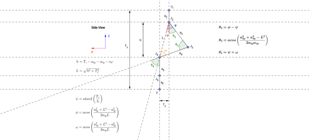
I found a geometrical solution to the IK by breaking the 3D problem down into two 2D problems:
Looking at the leg from the back/front, only joints 1 & 5 determine the offset along the world Y axis. The joints are equalised so that the foot is always facing perpendicular to the ground.
Looking at the leg sideways, the rest of the joints 2, 3 & 4 are calculated using mostly acos/atan2 functions. Note that the leg link lengths need to be projected onto the z-plane, which is why the a2p, a3p etc. notation is used.

Trigonometry based on front view.
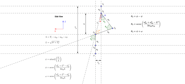
Trigonometry based on side view.
The test program now has controls for positioning a target for the foot to follow, based on the IK. This was very helpful for testing and debugging. A test function was also added which simply moves the target in an elliptical motion for the foot to follow. It is a very simple way of making the leg walk, but could be used as the foundation for a simply four-legged walking gait.
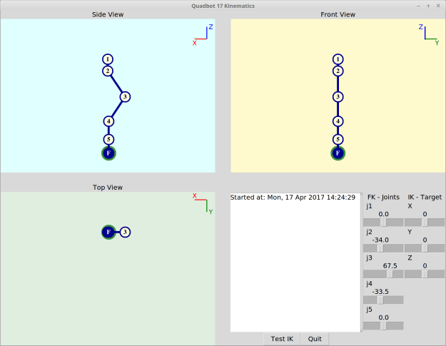
Kinematics test program updated with target visual and sliders.
Test of IK using elliptical motion target which the foot (F) follows.
The next tasks are to build the physical test rig, learn how to use the Arbotix controller and port the IK code to Arduino.
The kinematics are written in Python/TKInter, and code can be found on GitHub.
The geometrical drawings were made using the browser-based GeoGebra app.
The Forward Kinematics for the left leg of the Quadbot have been formalised, using modified Denavit-Hartenberg parameters and axes conventions.
I also made a simple Python applet to verify the maths and visualise the leg’s poses. I used Tkinter and three Canvas widgets to show orthogonal views.
The reason I am testing the maths in a quick Python program is that I want to be able to port them easily over to Arduino, as my latest aim is to drop the Raspberry Pi and A-Star 32U4 LV Pi expansion module (shown in some of the latest CAD models) in favour of trying out an ArbotiX controller. A benefit with the latter is that I wouldn’t need a Dynamixel-to-USB converter (e.g. USB2AX) or separate motor power supply.
Next up will be to work out the Inverse Kinematics.
| Link Twist |
Link Length |
Link Offset |
Joint Angle |
|
| j | alpha_i-1 | a_i-1 | d_i | theta_i |
| 1 | 0 | 0 | 0 | th_1 |
| 2 | pi/2 | 29.05 | 0 | th_2 – 34 |
| 3 | 0 | 76.919 | 0 | th_3 + 67.5 |
| 4 | 0 | 72.96 | 0 | th_4 |
| 5 | -pi/2 | 45.032 | 0 | th_5 |
D-H Parameters
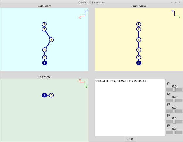
Quadbot kinematics applet, zeroed position

Quadbot kinematics applet, test position using sliders
A few and bits and pieces have been added to the model, along with some updates: Longer lower leg and cover, battery and battery compartment in rear body, main electronics boards, foot base and plate, and two ideas for sensors.
The lower legs were extended as initially the “knee” and “ankle” joints were too close. I think the new arrangement gives the leg better overall proportions.
As the battery pack has significant size and weight, its best to include in the design as early as possible. Originally neglected, I have now added a Turnigy 2200 mAh battery, and updated the rear bumper and bracket to accommodate it. Heat dissipation may be an issue, but I’ll leave it like this for now.
I have also measured the placement of the actuators in order to start thinking about the maths for the kinematics.
Some images of current progress:


I have tried two ideas for area scanners which could be the main “eyes” of the robot. One is the Kinect v2, and the other a Scanse Sweep.
The main advantages of the Sweep is that it is designed specifically for robotics, with a large range and operation at varying light levels. On its own it only scans in a plane by spinning 360°, however it can be turned into a spherical scanner with little effort. Added bonuses are a spherical scan mounting bracket designed specifically for Dynamixel servos, as well as ROS drivers! It is currently available only on pre-order on SparkFun.
The Kinect has a good resolution and is focused on tracking human subjects, being able to track 6 complete skeletons and 25 joints per person. However it only works optimally indoors and at short ranges directly in front of it. It is however significantly cheaper than the Sweep.
Below is a table comparing the important specs:
|
XBOX Kinect v2 |
Scanse Sweep |
|
|
Technology |
Time-of-Flight |
LiDAR |
|
Dimensions (mm) |
249 x 66 x 67 |
65 x 65 x 52.8 |
|
Weight (kg) |
1.4 |
0.12 |
|
Minimum Range (m) |
0.5 |
~0.1 |
|
Maximum Range (m) |
4.5 |
40 |
|
Sample rate (Hz) |
30 |
1000 |
|
Rotation rate (Hz) |
N/A |
1-10 |
|
FOV (°) |
70 x 60 |
360 (planar) |
|
Resolution |
512 x 424, ~ 7 x 7 pixels per ° |
1 cm |
|
Price (£) |
280 |
80 (32 for adaptor) |
Sources:
WordPress tip: One thing I really like about WordPress.com is that there are always ways around doing things that initially only seem possible with WordPress.org. Need to add a table into your post? Use Open Live Writer, make the table then copy-paste the table’s generated HTML source code!
The current estimated hardware costs are quite high, at around £2100. However about half this budget (£955) is due to the fact that I calculated the costs for the custom 3D printed parts by getting quotes from Shapeways. Getting them printed on a homemade 3D printer would reduce the cost significantly. The other large cost is naturally the 22 AX actuators at £790.
For anyone interested, the preliminary BOM can be downloaded here:
Quadbot 17 BOM – 2017-02-26.xlsx
That’s it for now!
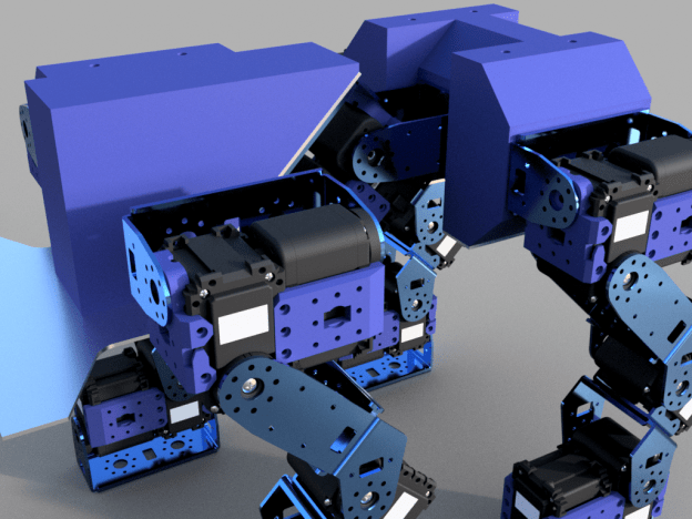
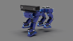
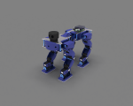
Here are some images of recent progress with the quadruped robot, taken as I familiarise with Autodesk Fusion 360:


