Force Sensing Resistors and Inertial Measurement Unit

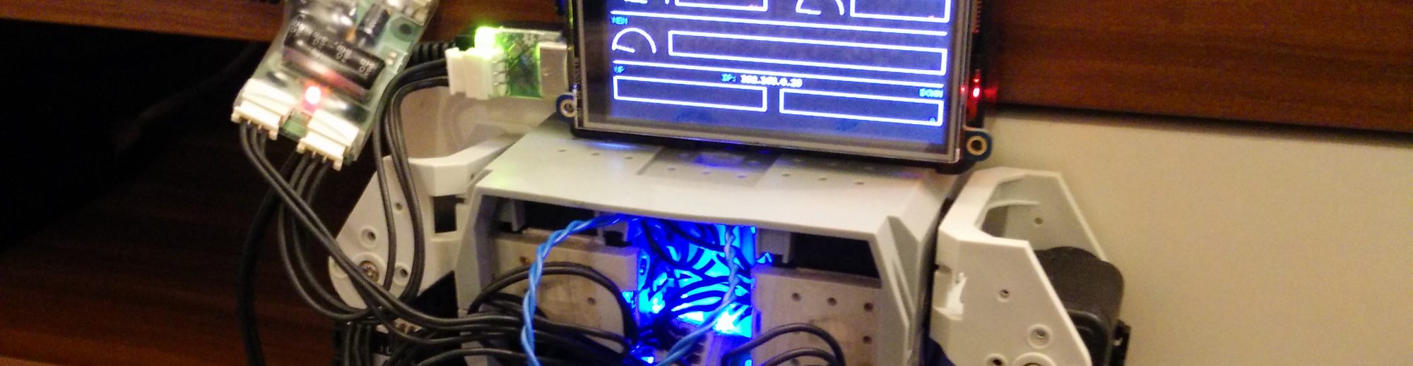
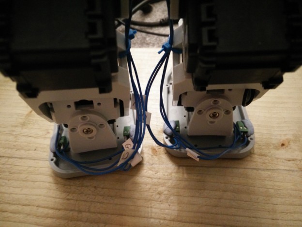
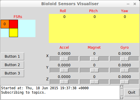
The first hardware parts to be tested were the inertial measurement unit (IMU) and the force sensing resistors (FSRs). The Arduino IDE was used for programming. The FSRs are straightforward analogue inputs, so I will concentrate on the IMU.

In order to be in line with the ROS coordinate frame conventions, the robot’s base frame will be in this orientation (right-hand rule):

• x axis: forward
• y axis: left
• z axis: up

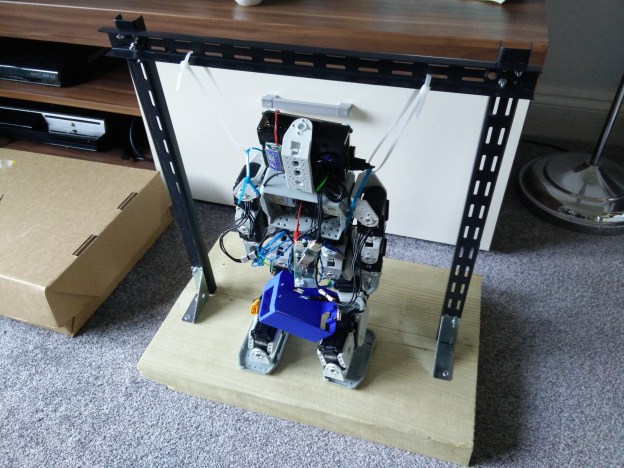
For now I am assuming the IMU is in the same orientation, but as it is not yet mounted to the robot, it might change later on. Again, in keeping with the ROS conventions on relationships beteen coordinate frames, the following transforms and their relationships have to be defined:

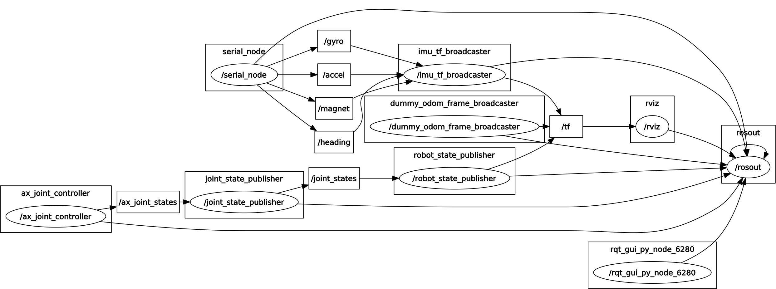
All these frames and their relationships can be easily managed using the ROS tf package.
I have added the imu_link to this chain, which represents the IMU’s orientation with respect to the odom frame. An additional link is also added to transform the standard base_link to the robot’s torso orientation. So the transform chain actually looks like this:

Calculating roll/pitch/yaw

I initially decided to let the A-Star (Arduino-compatible) board perform the IMU calculations and pass roll/pitch/yaw (RPY) values, and pass them as a ROS message to the PC. A ROS node will read these values and broadcast the transform from odom to imu_link using tf.

The IMU I am using, the MinIMU-9 v3 from Pololu, consists of an LSM303D accelometer-magnetometer chip and an L3GD20H gyro chip in one single package. The accelerometer, magnetometer and gyro are all three-axis types, providing 9 degrees of freedom and allow for a full representation of orientation in space. The data can be easily read using the provided Arduino libraries.

Rotations in Cartesian space will be represented in terms of intrinsic Euler angles, around the three orthogonal axes x, y and z of the IMU. As the order in which rotations are applied is important, I decided to use the standard “aerospace rotation sequence”, which has an easy mnemonic: An aeroplane yaws along the runway, then pitches during takeoff, and finally rolls to make a turn once it is airborne. The rotation sequence is thus:

• Rotation about z: yaw (±180°)
• Rotation about y: pitch (±90°)
• Rotation about x: roll (±180°)

Pitch has to be restricted to ±90° in order to represent any rotation with a single set of RPY values. The accelerometer alone can extract roll and pitch estimates, but not yaw, as the gravity vector doesn’t change when the IMU is rotated about the y axis. This is where the magnetometer (compass) comes in use.

Hence, using these accelerometer and magnetometer values, the IMU’s orientation can be fully described in space. However these measurements are very noisy, and should only be used as long-term estimates of orientation. Also, any accelerations due to movement and not just gravity add disturbances to the estimate. To compensate for this, the gyro readings can be used as a short term and more accurate representation orientation, as the gyro readings are more precise and not affected by external forces.

The complementary filter

Gyro measurements alone suffer from drift, so they have to be combined with the accelerometer/magnetometer readings to get a clean signal. A fairly simple way to do this is using what is known as a complementary filter. It can be implemented in code fairly simply, in the following way:

On every loop, the previous RPY values are updated with the new IMU readings. The complementary filter is essentially a high-pass filter on the gyro readings, and a low-pass filter on the accelerometer/magnetometer readings. is a filtering coefficient, which determines the time boundary between trusting the gyroscope vs trusting the accelerometer/magnetometer, defined as:

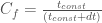
is the loop time, and is a time constant, which determines the length of recent history for which the gyro data takes precedence over the accelerometer/magnetometer data, in calculating the new values. I have set this to 1 second, so the accelerometer data from over a second ago will take precedence and correct any gyro drift. A good source of information on the complementary filter can be found here.

Issues with filtering roll/pitch/yaw values

However, when using RPY calculations, applying this filter is not so straightforward. Firstly, when the roll/yaw values cross over the ±180° point, the jump has to be taken into account otherwise it causes large erroneous jumps in the averaged value. This can be corrected fairly simply, however another problem is gimbal lock, which in this case is caused then the pitch crosses the +-pi/2 points (looking directly. This causes the roll/yaw values to jump abruptly, and as a result the IMU estimation “jumps” around the problem points. My attempt at solving this issue by resetting the estimated values whenever IMU was near the gimbal lock position was not very effective.

After a lot of frustration, I decided that learning how to reliably estimate position using quaternions was the way to go, although they may at first seem daunting. So at this point I abandoned any further experimentation using RPY calculations, however the work was a good introduction to the basics of the A-Star board and representing orientations using an IMU. The Arduino code is posted here for reference. Links to tutorials on using accelerometer and gyro measurements can be found in the comments.

Code (click to expand):

// Hardware:
// Pololu A-Star 32U4 Mini SV
// Pololu MinIMU-9 v3 (L3GD20H and LSM303D)
// Interlink FSR 400 Short (x6)

// Important! Define this before #include <ros.h>
#define USE_USBCON

#include <Wire.h>
#include <ros.h>
#include <std_msgs/Int16MultiArray.h>
#include <geometry_msgs/Vector3.h>
#include <AStar32U4Prime.h>
#include <LSM303.h>
#include <L3G.h>
#include <math.h>

// Set up the ros node and publishers
ros::NodeHandle nh;
std_msgs::Int16MultiArray msg_fsrs;
std_msgs::MultiArrayDimension fsrsDim;
ros::Publisher pub_fsrs("fsrs", &msg_fsrs);
geometry_msgs::Vector3 msg_rpy;
ros::Publisher pub_rpy("rpy", &msg_rpy);
unsigned long pubTimer = 0;

const int numOfFSRs = 6;
const int FSRPins[] = {A0, A1, A2, A3, A4, A5};
int FSRValue = 0;
LSM303 compass;
L3G gyro;
const int yellowLEDPin = IO_C7;  // 13
int LEDBright = 0;
int LEDDim = 5;
unsigned long LEDTimer = 0;

float aX = 0.0;
float aY = 0.0;
float aZ = 0.0;
float gX = 0.0;
float gY = 0.0;
float gZ = 0.0;
float accelRoll = 0.0;
float accelPitch = 0.0;
float magnetYaw = 0.0;
float roll = 0.0;
float pitch = 0.0;
float yaw = 0.0;
float accelNorm = 0.0;
int signOfz = 1;
int prevSignOfz = 1;
float dt = 0.0;
float prevt = 0.0;
float filterCoeff = 1.0;
float mu = 0.01;
float timeConst = 1.0;

void setup()
{
    // Array for FSRs
    msg_fsrs.layout.dim = &fsrsDim;
    msg_fsrs.layout.dim[0].label = "fsrs";
    msg_fsrs.layout.dim[0].size = numOfFSRs;
    msg_fsrs.layout.dim[0].stride = 1*numOfFSRs;
    msg_fsrs.layout.dim_length = 1;
    msg_fsrs.layout.data_offset = 0;
    msg_fsrs.data_length = numOfFSRs;
    msg_fsrs.data = (int16_t *)malloc(sizeof(int16_t)*numOfFSRs);

    nh.initNode();
    nh.advertise(pub_fsrs);
    nh.advertise(pub_rpy);

    // Wait until connected
    while (!nh.connected())
        nh.spinOnce();
    nh.loginfo("ROS startup complete");

    Wire.begin();

    // Enable pullup resistors
    for (int i=0; i<numOfFSRs; ++i)
        pinMode(FSRPins[i], INPUT_PULLUP);

    if (!compass.init())
    {
        nh.logerror("Failed to autodetect compass type!");
    }
    compass.enableDefault();

    // Compass calibration values
    compass.m_min = (LSM303::vector<int16_t>){-3441, -3292, -2594};
    compass.m_max = (LSM303::vector<int16_t>){+2371, +2361, +2328};

    if (!gyro.init())
    {
        nh.logerror("Failed to autodetect gyro type!");
    }
    gyro.enableDefault();

    pubTimer = millis();
    prevt = millis();
}

void loop()
{
    if (millis() > pubTimer)
    {
        for (int i=0; i<numOfFSRs; ++i)
        {
            FSRValue = analogRead(FSRPins[i]);
            msg_fsrs.data[i] = FSRValue;
            delay(2);  // Delay to allow ADC VRef to settle
        }

        compass.read();
        gyro.read();

        if (compass.a.z < 0)
            signOfz = -1;
        else
            signOfz = 1;

        // Compass - accelerometer:
        // 16-bit, default range +-2 g, sensitivity 0.061 mg/digit
        // 1 g = 9.80665 m/s/s
        // e.g. value for z axis in m/s/s will be: compass.a.z * 0.061 / 1000.0 * 9.80665
        //      value for z axis in g will be: compass.a.z * 0.061 / 1000.0
        //
        // http://www.analog.com/media/en/technical-documentation/application-notes/AN-1057.pdf
        //accelRoll = atan2( compass.a.y, sqrt(compass.a.x*compass.a.x + compass.a.z*compass.a.z) ) ;
        //accelPitch = atan2( compass.a.x, sqrt(compass.a.y*compass.a.y + compass.a.z*compass.a.z) );
        // Angle between gravity vector and z axis:
        //float accelFi = atan2( sqrt(compass.a.x*compass.a.x + compass.a.y*compass.a.y), compass.a.z );
        //
        // Alternative way:
        // http://www.freescale.com/files/sensors/doc/app_note/AN3461.pdf
        // Angles - Intrinsic rotations (rotating coordinate system)
        // fi: roll about x
        // theta: pitch about y
        // psi: yaw about z
        //
        // "Aerospace rotation sequence"
        // yaw, then pitch, then roll (matrices multiplied from right-to-left)
        // R_xyz = R_x(fi) * R_y(theta) * R_z(psi)
        //
        // Convert values to g
        aX = (float)(compass.a.x)*0.061/1000.0;
        aY = (float)(compass.a.y)*0.061/1000.0;
        aZ = (float)(compass.a.z)*0.061/1000.0;
        //accelRoll = atan2( aY, aZ );
        // Singularity workaround for roll:
        accelRoll  = atan2( aY, signOfz*sqrt(aZ*aZ + mu*aX*aX) );  // +-pi
        accelPitch = atan2( -aX, sqrt(aY*aY + aZ*aZ) );            // +-pi/2

        // Compass - magnetometer:
        // 16-bit, default range +-2 gauss, sensitivity 0.080 mgauss/digit
        // Heading from the LSM303D library is the angular difference in
        // the horizontal plane between the x axis and North, in degrees.
        // Convert value to rads, and change range to +-pi
        magnetYaw = - ( (float)(compass.heading())*M_PI/180.0 - M_PI );

        // Gyro:
        // 16-bit, default range +-245 dps (deg/sec), sensitivity 8.75 mdps/digit
        // Convert values to rads/sec
        gX = (float)(gyro.g.x)*0.00875*M_PI/180.0;
        gY = (float)(gyro.g.y)*0.00875*M_PI/180.0 * signOfz;
        gZ = (float)(gyro.g.z)*0.00875*M_PI/180.0;

        dt = (millis() - prevt)/1000.0;

        filterCoeff = 1.0;
        // If accel. vector magnitude seems correct, e.g. between 0.5 and 2 g, use the complementary filter
        // Else, only use gyro readings
        accelNorm = sqrt(aX*aX + aY*aY + aZ*aZ);
        if ( (0.5 < accelNorm) || (accelNorm > 2) )
            filterCoeff = timeConst / (timeConst + dt);

        // Gimbal lock: If pitch crosses +-pi/2 points (z axis crosses the horizontal plane), reset filter
        // Doesn't seem to work reliably!
        if ( (fabs(pitch - M_PI/2.0) < 0.1) && (signOfz != prevSignOfz) )
        {
            roll += signOfz*M_PI;
            yaw += signOfz*M_PI;
        }
        else
        {
            // Update roll/yaw values to deal with +-pi crossover point:
            if ( (roll - accelRoll) > M_PI )
                roll -= 2*M_PI;
            else if ( (roll - accelRoll) < - M_PI )
                roll += 2*M_PI;
            if ( (yaw - magnetYaw) > M_PI )
                yaw -= 2*M_PI;
            else if ( (yaw - magnetYaw) < - M_PI )
                yaw += 2*M_PI;

            // Complementary filter
            // https://scholar.google.co.uk/scholar?cluster=2292558248310865290
            roll  = filterCoeff*(roll  + gX*dt) + (1 - filterCoeff)*accelRoll;
            pitch = filterCoeff*(pitch + gY*dt) + (1 - filterCoeff)*accelPitch;
            yaw   = filterCoeff*(yaw   + gZ*dt) + (1 - filterCoeff)*magnetYaw;
        }

        roll  = fmod(roll,  2*M_PI);
        pitch = fmod(pitch,   M_PI);
        yaw   = fmod(yaw,   2*M_PI);

        msg_rpy.x = roll;
        msg_rpy.y = pitch;
        msg_rpy.z = yaw;

        pub_fsrs.publish(&msg_fsrs);
        pub_rpy.publish(&msg_rpy);

        prevSignOfz = signOfz;

        prevt = millis();

        pubTimer = millis() + 10;  // wait at least 10 msecs between publishing
    }

    // Pulse the LED
    if (millis() > LEDTimer)
    {
        LEDBright += LEDDim;
        analogWrite(yellowLEDPin, LEDBright);
        if (LEDBright == 0 || LEDBright == 255)
            LEDDim = -LEDDim;

        // 50 msec increments, 2 sec wait after each full cycle
        if (LEDBright != 0)
            LEDTimer = millis() + 50;
        else
            LEDTimer = millis() + 2000;
    }

    nh.spinOnce();
}